Help.

• Steps for analysing a target.  
• Screen layout.
• Using the controls, menus & buttons.
  • Input menus.
  • Output menus.
  • Image control buttons.
  • Target image controls.
• Interpreting the results.
  • Numerical results.
  • Graphical results.
• Average panel.

Steps for Analysing a Target.

1. Load in a JPEG (JPG) image from a digital camera.
2. Set the scale of the image to be analysed.
3. Indicate the bullet holes.
4. Save the analysis results.
5. That's it!
   

Image & Analysis Screen Layout.

IMAGE BUTTONS - used to identify the bullet holes and set the scale of the image. See "Using the Image Buttons".

IMAGE CONTROLS - the arrows and graticule are used to indicate the scale of the image and the Point of Aim. See "Using the Image Controls".

HEADER PANEL - enter the data relating to the shell under test. See "Header Panel and Menus".

SPREAD GRAPHICS - shows the graphical analysis of the group superimposed on the target image. See "Graphical group spread results". 

GROUP STATISTICS - shows the numerical analysis of the group See "Interpreting the results!"

Input Menus.

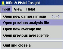
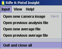
	Open a camera image of a target. Note that the image must be in JPEG format and at least 200 x 200 pixels in size.
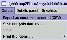
	Open a previously saved analysis file.
	Open a new window to allow multiple saved Analysis Files to be averaged. (see Average Panel.)
	Open a previously saved 'Average File'. (see Average Panel.)
	Closes all open windows and then quits the programme. Note that any windows that have been 'minimised' will remain open and the programme will not quit. These windows must be expanded and "Quit and close all" called again or each window should be closed individually.

Output Menus.

		Export as comma separated variables (CSV). Saves a simple text file to disk with all fields separated by commas. The "Export as CSV" of an Analysis File includes the numerical summary of the group as shown on screen, the user entered shell and gun details and also the shot  x-y coordinates using the same units of measurement (cm or inches) as used for the on-screen statistics.
		Save the analysis of the data with the option of renaming the file. Please note that only the Header Panel, Analysis Graphic and Analysis Panel are saved. The original image file from which the data are drawn is not saved.
		Save an analysis file using its current name without a prompt to rename the file.
		Print  . . . . ..
	Print the header panel (gun, shell, weather etc details ) and numerical analysis of the target and as much of the target image as possible using the current on-screen zoom setting. The 100%-10% contrast and "No target image" settings progressively grey-out the image to give the option of saving printer ink if there are large areas of black in the target image, for example large bulls-eye style targets.
		Print the target image and the spread graphics currently showing on the display screen. The print-out automatically resizes to fit a single page. The 100%-10% contrast and "No target image" settings progressively grey- out the image to give the option of saving printer ink if there are large areas of black in the target image, for example large bulls-eye style targets.

Header Panel and Menus.

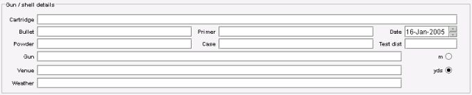
The header panel is for recording the test conditions. None of the fields affect the calculations. 

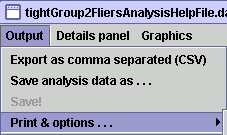
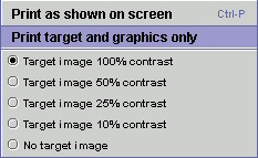
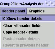
Once the shell and test conditions have been entered the header panel can be hidden from view to make available a larger screen area for working with the target image. A hidden header panel will still be shown on hard copy print-outs when using the Print as shown on screen option.

To speed the copying of details from one header panel to another during load development, details can be quickly copied to and from different panels as described below:

	Clears all the header panels with the exception of the date field. If the command was executed in error, the Revert to previous header command will return the header panel to its state when the clear command was executed (assuming the Paste header details command has not been executed after the clear command)..
	Copy the current header panel data into a hidden buffer for copying to other header panels. NB: If the date field has been altered make sure the new value entered has been validated by moving the cursor to another field.
	If header panel data has been copied from the current or another header panel it can be pasted into the current header panel.
	A copy of the old header panel data is held whenever the paste or clear command is used. This command returns the data to the header panel.

Image Buttons.

	Decrease / increase the size of the image. Does not affect any of the statistical calculations.
	Set the scale of the image. Drag the up/down arrows on the image to indicate a known vertical distance on the image and the left/right arrows to indicate a known horizontal distance. Move the graticule to indicate the point of aim.
	Horizontal / Vertical fields to enter the true distance indicated by the scale setting arrows.
	The distances may be input in imperial inches or metric cm. The calculated spread statistics of the group will use the same units.  (Note: If the units of measurement are changed the numerical group statistics will appear not to change. The reason for this is that the distance indicated by the scale arrows has also been converted to the new units.)
	Enters or exits the add annotations / notes mode. "Double clicking" the target image will open an editor box to allow notes to be entered. Double clicking an existing annotation will open it for editing or deletion. Clicking and holding the mouse over an existing annotation box and dragging the mouse will move the annotation box. (Note: The automatically generated annotation box showing the spread statistics cannot be deleted.)
	Add or delete bullet holes. When enabled clicking on the target image will add a hole shown as a blue marker. SHIFT+clicking over a blue hole mark will delete it. Two hole markers cannot be added directly on top of one another.

Target Image Controls.

	Manually added bullet hole. When in the pellet add mode clicking on the image adds a hole marker. Holes cannot be added directly on top of one another. "Shift-clicking" over a hole marker removes it.
	Define the top and bottom of a known vertical distance. Click-and-hold inside an arrow with the mouse and drag the arrow around the image. (Note: The vertical arrows allow a small misalignment to correct for any rotational errors incurred when taking the picture.)
	Define the left and right points of a known horizontal distance. Click-and-hold inside an arrow with the mouse and drag the arrow around the image. (Note: The horizontal arrows allow a small misalignment to correct for any rotational errors incurred when taking the picture.)
	Indicate the point of aim. Click-and-hold inside the graticule with the mouse and drag the centre of the graticule to the point of aim.

Analysis Panel - Interpreting the results!

Numerical group results.

See the table below for an explanation of the numbers. The colour coding for the numerical and graphical calculations is:

• Green for average spread and POI calculations;
• Red for extreme spread calculations;
• Orange for the string calculations.

Graphical group spread results.

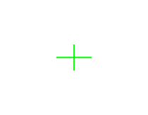
	The green cross shows the average Point of Impact (POI).  The numerical value is shown as "Average point of impact : horiz / vert". If this was to be calculated by hand it would be found by adding all the horizontal distances of the holes and then dividing by the number of holes to give the average horizontal position. The would be done for the vertical positions of the holes. This is also known as the mean average.
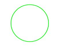
	The green circle or oval shows the average radius as measured from the average POI.  The numerical value is shown as "Average radius". If this was to be calculated by hand it would be found by measuring all the distances from the previously calculated average POI to each hole, adding all the distances together and dividing by the number of holes.
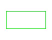
	The green rectangle shows the average horizontal and vertical spread. These are the +/- one standard deviations horizontally and vertically. The numerical value is shown as "Average spread : horiz / vert". If these were to be calculated by hand the method would be as follows: For each hole measure the horizontal (or vertical) distance from the average POI and square the distance. Add all the squared distances and divide by the number of holes minus one. The square root of this number gives what is known as the horizontal (or vertical) standard deviation of the group.
	The red line between two points shows the maximum spread between two points. This is the traditional measure of group size. The numerical value is shown as "Extreme spread between two points".
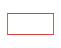
	The red rectangle shows the extreme horizontal and vertical spreads. The numerical values are shown for the horizontal and vertical separately as follows: "Extreme horizontal spread : total / left / right" "Extreme vertical spread : total / high / low" Note that the total extreme spread gives the maximum horizontal or vertical distance between two or more points. The left / right and high / low figures are calculated compared to the average POI.
	The red circle / oval shows the extreme radius. This shows the maximum distance of a hole from the average POI (the green cross) and treats this distance as a radius and draws a circle with this radius about the average POI. The numerical value is shown as "Extreme radius".
	The orange lines show the "string" distances. The total string distance is the sum of all the distances from the Point of Aim (POA).  The numerical values for the string measurements are shown as "String length : total / max / ave". These show the total string distance, the maximum and average distance of each hole from the POA. The average string distance allows easier comparisons between groups containing different numbers of shots.
	The scale markers are used to show a known vertical and horizontal distance on the real target. If the camera is not perfectly aligned with the target these horizontal and vertical distances will not be horizontal and vertical on-screen. The scale markers can accommodate this and all the results are corrected for the rotational error. i.e. the "horizontal" spread is shown not as horizontal with the screen, but with the horizontal indicated by the scale markers. Experiment with extreme rotations to see how it works. Up to 5-degrees of correction can be accommodated.

Average Panel.

Menu functions unique to the Average Panel.

Interpreting the Average Panel numerical results.

Averaging allows analysis of multiple groups/targets. If for example over a whole year of varying weather conditions and altitudes test groups had been taken, they could all be added together to see which shell gave the best performance over real-world usage conditions. Rifle & Pistol Insight offers two alternatives for handling averaged groups - if you use them, make sure you understand them! See: Interpreting the Average Panel numerical results.

HEADER PANEL  - this is the same as in the single target analysis panel.

LIST OF ANALYSIS FILES - As Analysis Files are added to the average panel, their name and some key features from their header panels are shown. This allows a quick visual check that all data to be averaged comes from the same gun or cartridge. If the header panel is empty, the first Analysis File or Average File added will donate it's header panel contents to the current one.

FOOTER PANEL - clicking on a file in the list of analysis files causes the header panel of the analysis file to be displayed in the footer panel. From here it can be copied and then pasted to the current header panel. See Copy footer details.

AVERAGE OF SHOTS, AVERAGE OF GROUPS - are similar to the single target analysis panel but need some special explanation: See Interpreting the Average Panel Results.

Additional Menu Functions of the Average Panel.

	Clicking on a file in the LIST OF ANALYSIS FILES will cause the header panel originally associated with this file to be displayed at the bottom of the screen in the FOOTER PANEL. Selecting "Copy footer details" in the drop down menu will allow these details to be copied to the header panel of the current averaging screen or to another single target analysis screen.
	Add an earlier Analysis File to this Average Panel.
	Add an earlier Average File to this Average Panel.

Delete the file(s) highlighted in the list of the Average Panel. It is possible to highlight multiple files in the list of analysis files. Dragging the mouse across multiple lines a selects continuous series. Pressing the "Control" (CNTRL) key while clicking the mouse on lines allows a discontinuous series to be selected. 

Interpreting the Average Panel Results.

The AVERAGE OF SHOTS and AVERAGE OF GROUPS look very similar display with almost the same fields, but the number will most times be very different. The different ways they handle the data needs to be understood.

To help with examples, consider two five shot Groups A and B. Group A has a 1" average spread and is around the POA. Group B has a similar average spread of 1", but the POI has been set 6" above the POA.

The AVERAGE OF SHOTS is the easiest to understand. This treats all the shots as though they had been fired at a single target with a single point of aim (POA). It takes all the positions of all the points in all of the analysis files and performs the spread calculations as though it was dealing with one large analysis file. Using the two example groups, the average spread would be reported as very much larger than 1" because of the 6" shift of the sights. For fixed sight guns this averaging method shows how the gun groups long term or over several targets or varying weather conditions.

The AVERAGE OF GROUPS is better for when big systematic changes have been made such as the sights being adjusted. Rather than take the raw shot position and calculate everything afresh, it takes the previously calculated spread and POI figures from the analysis files and averages these. In this way, the average spread of Group A and Group B would be reported as approximately 1" - which is what is wanted in this case. The average of the POIs is calculated and with this example would be approximately 3" (the average of ~0" and ~6"). Similarly, all the other spread figures are averages of those previously calculated. The averaging method takes account of groups with different numbers of shots. The spread statistics of a group of 10 shots would be weighted twice as high as a group of only 5 shots.

(c) A C Jones    January 2005